| Homepage Alexander Schatten - Genetic Algorithms Short Tutorial |
|
|
|
|
|
|
|
|
|
|
| > Home > Resources > Genetic Algorithms Short Tutorial |
Genetic Algorithms Short Tutorial1. IntroductionThe idea behind GA's is to extract optimization strategies nature uses successfully - known as Darwinian Evolution - and transform them for application in mathematical optimization theory to find the global optimum in a defined phase space. One could imagine a population of individual "explorers" sent into the optimization phase-space. Each explorer is defined by its genes, what means, its position inside the phase-space is coded in his genes. Every explorer has the duty to find a value of the quality of his position in the phase space. (Consider the phase-space being a number of variables in some technological process, the value of quality of any position in the phase space - in other words: any set of the variables - can be expressed by the yield of the desired chemical product.) Then the struggle of "life" begins. The three fundamental principles are Only explorers (= genes) sitting on the best places will reproduce and create a new population. This is performed in the second step (Mating/Crossover). The "hope" behind this part of the algorithm is, that "good" sections of two parents will be recombined to yet better fitting children. In fact, many of the created children will not be successful (as in biological evolution), but a few children will indeed fulfill this hope. These "good" sections are named in some publications as building blocks. Now there appears a problem. Repeating these steps, no new area would be explored. The two former steps would only exploit the already known regions in the phase space, which could lead to premature convergence of the algorithm with the consequence of missing the global optimum by exploiting some local optimumy. The third step - the Mutation ensures the necessary accidental effects. One can imagine the new population being mixed up a little bit to bring some new information into this set of genes. Off course this has to happen in a well-balanced way! Whereas in biology a gene is described as a macro-molecule with four different bases to code the genetic information, a gene in genetic algorithms is usually defined as a bitstring (a sequence of b 1´s and 0´s). Don´t project results obtained from GA-performance or different qualities of algorithm types to biological/genetic procedures. The aim of GA´s is not to model genetics or biological evolution! Consider GA´s as a kind of bionic in trying to extract successful natural strategies for mathematical problems. 2. Algorithm
2.1 Initial PopulationAs described above, a gene is a string of bits. The initial population of genes (bitstrings) is usually created randomly. The length of the bitstring is depending on the problem to be solved (see section Applications).2.2 SelectionSelection means to extract a subset of genes from an existing (in the first step, from the initial -) population, according to any definition of quality. In fact, every gene must have a meaning, so one can derive any kind of a quality measurement from it - a "value". Following this quality "value" (fitness), Selection can be performed e.g. by Selection proportional to fitness:
But we shoult not forget, that there are a lot of different implementations of these algorithms. For example the Selection module is not always creating constant population sizes. In some implementations the size of the population in dynamic. Furthermore, there exist a lot of other types of selection algorithms (the most important ones are: Proportional Fitness, Binary Tournament, Rank Based). I restrict myself to describe just the most common implementations in this short article. To get a deeper insight to this topic take a look to the Recommended Reading section. 2.3 Mating/Crossover
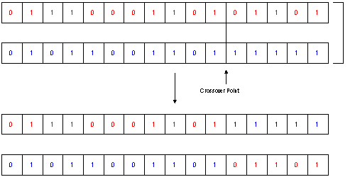
The next steps in creating a new population are the Mating and Crossover: As described in the previous section there exist also a lot of different types of Mating/Crossover. One easy to understand type is the random mating with a defined probability and the b_nX crossover type. This type is described most often, as the parallel to the Crossing Over in genetics is evident:
In fact, more often a slightly different algorithm called b_uX is used. This crossover type usually offers higher performance in the search.
2.4 Mutation
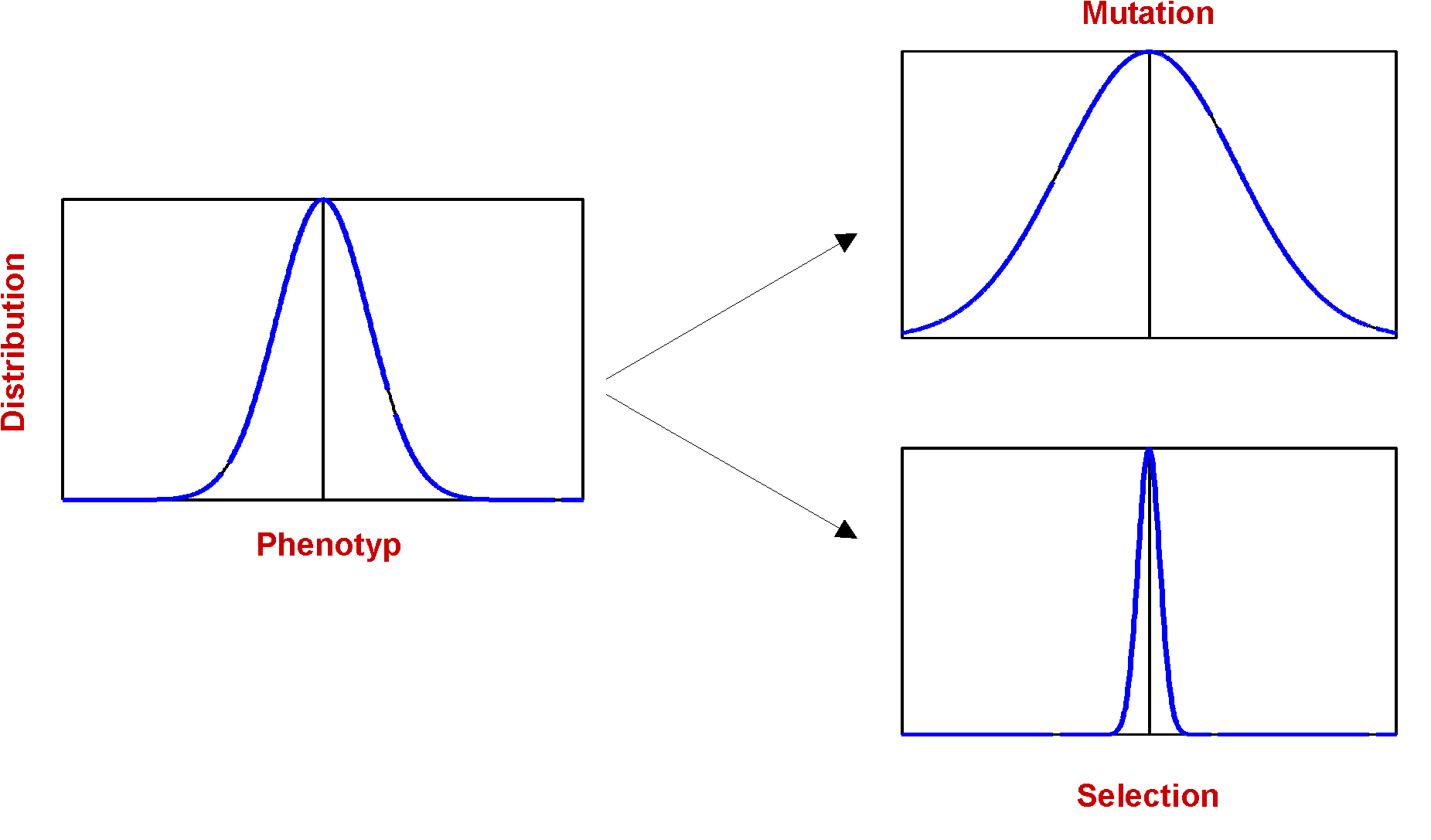
The last step is the Mutation, with the sense of adding some effect of exploration of the phase-space to the algorithm. The implementation of Mutation is - compared to the other modules - fairly trivial: Each bit in every gene has a defined Probability P to get inverted. The effect of mutation is in some way a antagonist to selection:
3. Application(s) - Coding Problems3.1 IntroductionThree important applications will be mentioned here:
3.2 Parameter EstimationConsider a statistical model f(x1, x2, ... xi) with parameters (a1, a2, ... aj) and the data set (y1, y2, ... yk). The task is to calculate the estimated parameters (a'1, a'2, ... a'j ). In many cases the calculation of the estimated parameters is possible with an mathematically derived formula (see Linear Regression). But in many interesting instances this is not possible. Furthermore, every time varying the model, a new derivation of the solution is necessary. Using GA´s can be a good solution in these (often rather complex) problems.
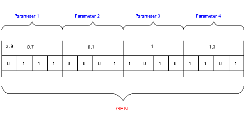
Now the problem arises, that the model is described by a set of (usually) real - type variables, but genetic algorithms work with a bitstring as phase-space representation! The usual way to solve this issue is (example see fig.4):
Remark: Usually not the binary representation is used, but the Gray-code representation (see Vankeerberghen et.al.) How to use the algorithm?
Remark: As it is not easily possible to define a threshold of fitness to stop iteration (as the search-space is not known in detail) in many cases, often a defined number of iterations (= generations) is calculated. It is advisable to perform more than one GA-calculation of one fit to increase the probability, that the GA - had found the global optimum. In a more general way, the problem could be described as follows: Imagine a black-box with n - knobs, and one display in front of it, that shows a value (= a fitness!). The position of the knobs is correlated in some way with the value shown in the display (but not necessarily described in detail!). The duty is to turn these knobs with a good strategy to find the position showing the highest (or equivalently the lowest) value in the display. This good strategy can be using a genetic algorithm. So - in general - every problem one can formulate in this "black-box" way, giving a response to a set of variables (or a bitstring) can be optimized (solved) using a genetic algorithm! 3.3 Subset SelectionConsider a set of items (e.g. lots of data acquired with a multi-sensor array, spectroscopical data as IR- or MS - spectra, ...). Reducing the size of the dataset by extracting a subset, containing the essential information for some application (recognition of functional groups, detection of pesticides) is called a Subset Selection problem. Two ways of coding a Subset Selection problem are common:
3.4 SequencingFinding an good or optimal order of a given set of items is called a sequencing problem (E.g. Traveling Salesman problems, finding optimal order of chromatographic columns, ...). A representation of the problem could be a permutation of numerical elements (e.g. 4 3 6 1 2 5). A problem in implementation is, that (as in some representations of Subset Selection problems) each element has to occur precisely once! 4. Recommended Reading4.1 Books
4.2 Articles
|


